Convex Hull Algorithms: Jarvis's March

Convex Hull

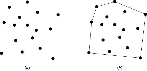
A convex hull of a given set of points is the smallest convex polygon containing the points. Intuitively, the convex hull is what you get by driving a nail into the plane at each point and then wrapping a piece of string around the nails. In the figure below, figure (a) shows a set of points and figure (b) shows the corresponding convex hull.

Convex Hull is useful in many areas including computer visualization, pathfinding, geographical information system, visual pattern matching, etc. In this article and three subsequent articles, I shall talk about the algorithms for calculating convex hull of a given set of points. Let’s talk about one of the fundamental algorithms for calculating convex hull known as Jarvis’s March algorithm.

Jarvis’s March

Please visit the article below before going further into the Jarvis’s march algorithm.

1. Determine if two consecutive segments turn left or right

Jarvis’s march algorithm uses a process called gift wrapping to find the convex hull. It is one of the simplest algorithms for computing convex hull. The working of Jarvis’s march resembles the working of selection sort. In selection sort, in each pass, we find the smallest number and add it to the sorted list. Similarly, in Jarvis’s march, we find the leftmost point and add it to the convex hull vertices in each pass. The step by step working of Jarvis’s march algorithm is given below.

1. From the given set of points $P$, we find a point with minimum x-coordinates ( or leftmost point with reference to the x-axis). Let’s call this point $l$. Since this point is guaranteed to be in the convex hull, we add this point to the list of convex hull vertices.
2. From $l$, find the leftmost point. For this, we do the following. We select the vertex following $l$ and call it $q$. We check if $q$ is turning right from the line joining $l$ and every other point one at a time. If $q$ is turning right, we move $q$ to the point from where it was turning right. This way we move $q$ towards left in each iteration and finally stop when $q$ is in the leftmost position from $l$. We add $q$ to the list of convex hull vertices.
3. Now $q$ becomes $l$ and we repeat the step (2).
4. Repeat step (2) and (3) until we reach the point where we started.

After the execution of this algorithm, we should get the correct convex hull.

Program

The python implementation of the Jarvis’s algorithm is given below.

1
2
3
4
5
6
7
8
9
10
11
12
13
14
15
16
17
18
19
20
21
22
23
24
25

def jarvis_march(points):
    # find the leftmost point
    a =  min(points, key = lambda point: point.x)
    index = points.index(a)
    
    # selection sort
    l = index
    result = []
    result.append(a)
    while (True):
        q = (l + 1) % len(points)
        for i in range(len(points)):
            if i == l:
                continue
            # find the greatest left turn
            # in case of collinearity, consider the farthest point
            d = direction(points[l], points[i], points[q])
            if d > 0 or (d == 0 and distance_sq(points[i], points[l]) > distance_sq(points[q], points[l])):
                q = i
        l = q
        if l == index:
            break
        result.append(points[q])

    return result

result holds the convex hull vertices. In the next section, I will show the execution trace of this program.

Execution Trace

The figure below shows a given set of points for this execution trace.

The program first finds the leftmost point by sorting the points on x-coordinates. The leftmost point for the above set of points is $l = (0, 0)$. We insert the point $(0, 0)$ into the convex hull vertices as shown by the green circle in the figure below.

Next we find the left most point from point $l = (0, 0)$. The step by step process of finding the left most point from $l = (0, 0)$ is given below.

1. We pick a point following $l$ and call it $q$. Let $q$ be the point $(3, 3)$ (You can pick any point, generally we pick next of $l$ in array of points).
2. Let all other points except $l$ and $q$ be $i$. Now we check whether the sequence of points $(l, i, q)$ turns right. If it turns right, we replace $q$ by $i$ and repeat the same process for remaining points.
3. Let $i = (7, 0)$. The sequence ((0, 0), (7, 0), (3, 3)) turns left. Since we only care about right turn, we don’t do anything in this case and simply move on.
4. Let next $i = (3, 1)$. The sequence ((0, 0), (3, 1), (3, 3)) turns left and we move on without doing anything.
5. Let next $i = (5, 2)$. The sequence ((0, 0), (5, 2), (3, 3)) again turns left and we move on.
6. Next $i = (5, 5)$. The sequence ((0, 0), (5, 2), (3, 3)) is collinear. In the case of collinear, we replace $q$ with $i$ only if distance between $l$ and $i$ is greater than distance between $q$ and $l$. In this case the distance between $(0, 0)$ and $(5, 5)$ is greater than the distance between $(0, 0)$ and $(3, 3)$ we replace $q$ with point $(5, 5)$.
7. Let next $i = (1, 4)$. The sequence ((0, 0), (1, 4), (5, 5)) turns right. We replace $q$ by point $(1, 4)$.
8. Finally the only choice for $i$ is $(9, 6)$. The sequence ((0, 0), (9, 6), (1, 4)) turns left. So we do nothing. We went through all the points and now $q = (1, 4)$ is the left most point.

We add point $(1, 4)$ to the convex hull.

Next, we find the leftmost point from the point $(1, 4)$ following the steps 1 - 8 mentioned above. If we follow all the steps, the leftmost point will be $(9, 6)$.

Using the same process, the leftmost point from $(9, 6)$ will be the point $(7, 0)$.

Finally from $(7, 0)$ we compute the leftmost point. The leftmost point from $(7, 0)$ will be the point (0, 0). Since $(0, 0)$ is already in the convex hull, the algorithm stops.

Complexity

The algorithm spends $O(n)$ time on each convex hull vertex. If there are $h$ convex hull vertices, the total time complexity of the algorithm would be $O(nh)$. Since $h$ is the number of output of the algorithm, this algorithm is also called output sensitive algorithm since the complexity also depends on the number of output.

References

1. Cormen, T. H., Leiserson, C. E., Rivest, R. L., & Stein, C. (n.d.). Introduction to algorithms (3rd ed.). The MIT Press.
2. Briquet, C. (n.d.). Introduction to Convex Hull Applications. Lecture. Retrieved August 23, 2018, from http://www.montefiore.ulg.ac.be/~briquet/algo3-chull-20070206.pdf
3. Erickson, J. (n.d.). Convex Hulls. Lecture. Retrieved August 23, 2018, from http://jeffe.cs.illinois.edu/teaching/373/notes/x05-convexhull.pdf
4. Mount, D. M. (n.d.). CMSC 754 Computational Geometry. Lecture. Retrieved August 23, 2018, from https://www.cs.umd.edu/class/spring2012/cmsc754/Lects/cmsc754-lects.pdf