Binary Trees

Introduction

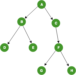
The binary trees are a type of tree where each node has maximum two degree. That means each node can have at most 2 child nodes. Binary trees are an extremely useful data structure in computer science. Figure 1 shows an example of a binary tree with 8 nodes.

The child node in the left of a node is called a left-child and the child node in the right is called a right-child. When there is only one child we can call it left-child. The leaf nodes do not have any child nodes.

Types of a binary tree

All the major types of a binary tree are explained in detail below.

Rooted Binary Tree

A binary tree with a root node and other nodes. Each node in a rooted binary tree has at most 2 children. Figure 1 is an example of a rooted binary tree.

Full Binary Tree

A full binary tree is a tree in which each node has either 0 or 2 children. The leaf nodes have 0 children and all other nodes have exactly 2 children. Figure 2 shows an example of a full binary tree.

In a full binary tree, the number of leaf nodes = number of internal nodes + 1.

Complete Binary Tree

A complete binary tree is a tree in which every level, except possibly the last, is filled. The nodes in the last level are filled from left to right.

Properties of a complete binary tree

1. The last level of a complete binary tree
   can have 1 to 2^h nodes where h is the height of the tree.
2. The number of internal nodes is the floor of n/2, where n is the total number of nodes.

Perfect Binary Tree

A perfect binary tree is a tree where all the interior nodes have 2 children and all the leaf nodes are on the same level.

Properties of a perfect binary tree

1. The number of leaf nodes = (n + 1)/2, where n is the total number of nodes.
2. The total number of nodes = 2^{h + 1} - 1, where h is the height of the tree.

Balanced Binary Tree

A balanced binary tree is a binary tree where the height of the left and the right subtree is differed by at most 1. This must be valid for each subtree. Examples of a balanced binary tree include AVL tree, Red-Black Tree, 2/3 Tree etc. One of the interesting property of a balanced tree is that the height of the tree is O(log n) which gives a guarantee that the insertion, deletion, and search operations are efficient.

Representation

There is two popular representation of a binary tree. One is the array representation and another is the linked list representation.

Using array

A binary tree can be implemented efficiently using an array. The array representation is most suited for a complete binary tree where the waste of the memory is minimum. We need to allocate 2^h+1 - 1 array items, where h is the height of the tree, that can fit any kind of binary tree. If i is the index of a parent, then the index of the left child is 2i + 1 and the index of the right child is 2i + 2. Fig 6 shows a binary tree and corresponding array representation.

Using linked list

In linked list representation, each node of the tree holds the reference for left and right child. Figure 7 shows a binary tree and its representation using the linked list.

As you can see in the figure, all the leaf nodes’ references point to a null pointer. More than half of the total nodes of a binary tree point to the null reference which is a huge waste of memory. This memory waste can be avoided using a Threaded Binary Tree.

Traversals

There are two types of traversal in a tree: (1) depth-first traversal and (2) breadth-first traversal.

Depth-first traversal

In depth-first traversal, we visit the child nodes before visiting the next sibling. In this way, we go deeper and deeper until there is no more child node left (i.e. we reach the leaf node). The algorithm for depth-first traversal is given below.

At node N, 
(1) Recursively traverse its left subtree.
(2) Recursively traverse its right subtree.
(3) Visit the node N itself.

Depending upon the order in which these operations occur, breadth-first traversal can be further divided into three categories.

1. Pre-Order traversal: We visit the root node first, then recursively traverse the left subtree and recursively traverse the right subtree. The pseudocode is given below.

   procedure pre-order(node) {
       if (node is not null) {
           print node.data;
           pre-order(node.leftnode);
           pre-order(node.rightnode);
       }
   }
   

   The pre-order traversal on the binary tree given in figure 1 is : A, B, D, E, C, F ,G, H.

2. In-Order traversal: We visit the left subtree recursively, visit the node and finally visit the right subtree. The pseudocode is given below.

   procedure in-order(node) {
       if (node is not null) {
           in-order(node.leftnode);
           print node.data;
           in-order(node.rightnode);
       }
   }
   

   The in-order traversal on the binary tree given in figure 1 is : D, B, E, A, G, F, H, C

3. Post-Order traversal: We visit the left subtree recursively, visit the right subtree recursively and finally visit the node. The pseudocode is given below.

   procedure post-order(node) {
       if (node is not null) {
           post-order(node.leftnode);
           post-order(node.rightnode);
           print node.data;
       }
   }
   

   The post-order traversal on the binary tree given in figure 1 is: D, E, B, G, H, F, C, A

Breadth-first traversal

It is also known as level-order traversal. In this traversal, we visit every node of a level before going to the lower level. The pseudocode for level-order traversal is given below.

procedure level-order(node) {
    queue.enqueue(node);
    
        while (queue is not empty) {
          node = queue.dequeue();
          if (node is not null) {
            print node.data;
            queue.enqueue(node.leftnode);
            queue.enqueue(node.rightnode);
          }
        }
}

The level-order traversal on the tree given in figure 1 is: A, B, C, D, E, F, G, H. This is illustrated in figure 8.